Compensating for coarticulation during phonetic category acquisition

• Naomi Feldman

Introduction

Recent models of phonetic category acquisition have taken a Mixture of Gaussians approach, in which Gaussian categories are chosen to best fit the distribution of speech sounds in the input, where the input typically consists of isolated speech sounds [1] [2] [3]. One limitation of these approaches is that they do not take into account predictable phonetic variability that is based on context. In actual speech, the acoustic realizations of a phoneme depend on the identities of neighboring sounds, due to coarticulation with these sounds (e.g., as demonstrated in [4] ). This presents a challenge for models of phonetic category acquisition that assume context-independent Gaussian distributions of sounds.

最近の音素カテゴリ獲得のモデルはガウス混合分布アプローチが取られている. このモデルにおいては分離された発話音声からなる典型的なインプットの発話音声の分布に最もよくフィットするガウシアンのカテゴリが選択される. これらのアプローチの限界は,コンテクストに基づく音声的な分散を考慮することができないことである. 実際の発話においては, コーティキュレーションがあるため, 音響的な音素の実体は近隣の音の特性に依存する. 本研究ではコンテクストに独立した音声のガウス分布を仮定した音素カテゴリ獲得モデルの変化を示す.

A more realistic model of phonetic category acquisition should take account of dependencies between neighboring acoustic values that arise due to factors such as gestural overlap and articulatory ease. Despite extensive research on the conditions under which people and animals compensate for coarticulation in speech perception, the problem has only recently begun to be addressed in the context of phonetic category acquisition. There has been a first attempt at solving this problem [5] , in which it is assumed that a learner needs to figure out the direction and magnitude of the shift in acoustic values that occurs in a particular context. This is done by taking the mean of all sound that occur in that context, and comparing it to the mean of all sounds that occur in other contexts.

音素カテゴリ獲得のより現実的なモデルは身振りの重複や音調的容易さのような要素のために起きる近隣の音響的値間の依存度を考慮するべきである. 人間や動物の音声知覚におけるコーアティキュレーションの補償における状態に関する広範囲な研究にもかかわらず, 音素カテゴリの獲得のコンテキストの特定を開始されたのは最近である. この問題の解決する最初の試みは存在し [5] , この研究では学習者が特定のコンテクストにおいて生じる音響的値の遷移の方向と大きさを理解する必要があると仮定している. これは, このコンテキストに生じたすべての音声の平均値を取得し,他のコンテキストで生じるすべての音声の平均とその音声を比較することで行った.

The authors demonstrate that correcting for this shift in the acoustic values makes it easier for a learner to recover a set of Gaussian phonetic categories from acoustic data. However, there is a circularity here, as categories must be known in order to pick out a particular phonological context that would cause an acoustic shift. Thus, it would be desirable for an algorithm to learn both layers of structure simultaneously. As a first step, this paper explores the category learning problem in a system where coarticulatory influences are present, but where the parametric form of these coarticulatory influences is assumed to be known.

作者はこの遷移の音響的値が学習者が音響データからガウシアンの音素カテゴリの再現することを容易にすることで, 正しさを示している. しかし, 音響的遷移を引き起こす特定の音韻的なコンテキストをピックアウトするためにカテゴリを知らなくてはいけないため, ここには矛盾が存在する. したがって, 両方のレイヤーを同時に学習するためのアルゴリズムが望ましい. 最初のステップとして, 本稿ではコーアティキュレーションの影響が存在し,かつ,その値のパラメータが既知であると仮定されるシステムのカテゴリ学習問題を調査した.

Phonological Constraints in Exponential Family Models

Phonological constraints were first proposed to be characterized by weighted harmony functions in Harmonic Grammar [6] . Phonetic productions of words in this framework are selected to best satisfy a set of weighted constraints, given the underlying phonological properties of those words. Constraints relate underlying properties to phonetic surface properties (e.g., a constraint would assign higher probability to a /p/ pronounced as [p], as opposed to [b]) and favor certain surface properties over others (e.g., a higher probability is assigned to CV syllables than to CCV syllables). This was later put into a maximum entropy learning framework [7] , where weights are learned for each constraint to maximize the likelihood of a set of training data. In this work, each function \(\phi\) (x) corresponds to a count of the number of times a particular constraint had been violated.

音素カテゴリは Harmonic Grammar [6] において, 重み付けられた調和関数によって決定するために最初に提案された. このフレームワークにおいて,単語の音声学的発声は最も妥当な重み付けられた拘束のセットを選択し,それらの単語の

注釈

Harmonic Grammar

Harmonic Grammar is a linguistic model proposed by Geraldine Legendre, Yoshiro Miyata, and Paul Smolensky in 1990. It is a connectionist approach to modeling linguistic well-formedness.

More recently, the same sort of constraint-based framework has been suggested to be useful for characterizing gradient phonetic effects. Flemming [8] proposed constraints that favor acoustic values similar to a given target production, and also favor similar acoustic values in neighboring speech sounds. Specifically, a speaker is assumed to be minimizing the weighted squared error terms

(1)\[\begin{eqnarray} \theta_1(\omega_1−\mu_1)^2 \end{eqnarray}\]

(2)\[\begin{eqnarray} \theta_2(\omega_1−\mu_1)^2 \end{eqnarray}\]

(3)\[\begin{eqnarray} \theta_3(\omega_1−\omega_2)^2 \end{eqnarray}\]

where each \(\theta\) term is the corresponding weight for a particular constraint, the w terms are the acoustic realizations of neighboring phonemes, and the \(\mu\) terms are targets for specific phonological categories.

This weighted sum squared error cost function corresponds to a particular type of pairwise undirected graphical model (Figure 1). In particular, if the squared error cost functions correspond to the log likelihood of a particular set of values for \(\omega_1\) and \(\omega_2\) , then the potential functions between each 1 pair of nodes are simply Gaussians with variance \(\frac{1}{2\theta}\).

Figure 1: The graphical model corresponding to the model used in [8] .

This problem can be generalized to a series of \(N\) acoustic values, where local potentials are Gaussian around the corresponding category mean \(\mu_c\) with variance \(\Sigma_C\) specific to that category, all pairwise potentials between neighboring acoustic values are Gaussian with common variance \(\Sigma_S\) . The conditional probability \(p(w|z)\) can be expressed as

(4)\[\begin{eqnarray} p(\omega|z) \propto \exp\left\{ - \frac{1}{2} \left[ \sum_{i=1}^{N}(\omega_i - \mu_{zi})^{T\sum_{zi}^{-1}}(\omega_i -\mu_{zi}) + \sum_{i=1}^{N-1}(\omega_i-\omega_{i+1})^{T\sum_{S}^{-1}}(\omega_i - \omega_{i+1}) \right] \right\} \end{eqnarray}\]

This can equivalently be expressed in the information form

(5)\[\begin{eqnarray} p(\omega | z) \propto \exp \left\{ - \frac{1}{2}\omega^TJ\omega + h^T\omega \right\} \end{eqnarray}\]

where each diagonal entry in the matrix \(J\) is \(\sum_{zi}^{-1} + 2\sum_{S}^{-1}\) , except the first and last diagonal entries which are \(\sum_{zi}^{-1} +\sum_{S}^{-1}\) , and the off-diagonal entries are \(−\sum_{S}^{-1}\) for neighboring sounds, zero otherwise.

Each entry in the vector \(h\) is equal to \(\sum_{zi}^{-1}\mu_{zi}\)

The acoustic values \(w_i\) are jointly Gaussian and their marginals can be computed straightforwardly using Gaussian belief propagation. Given category assignments and category parameters, the factor graph is simply a chain with local node potentials and pairwise potentials. The messages originate at the ends of the chain at the variable nodes. Messages from variable nodes to factor nodes are

(6)\[\hat{J_{i\j}} = \sum_{zi}^{-1} + \sum_{S}^{-1} + J_{k \to i} \mathrm{\ for\ } i = 1, N\]

(7)\[\begin{split}\hat{J_{i\j}} &= \sum_{zi}^{-1} + 2\sum_{S}^{-1} + J_{k \to i} \mathrm{\ for\ all\ other\ i}\\ \hat{h}_{i\j} &= \sum_{zi}^{-1}\mu_{zi} + h_{k \to i}\end{split}\]

where the chain structure ensures that there is at most one incoming message to take into account. Messages from factor nodes to variable nodes take the form of

(8)\[J_{i \to j} = -\sum_{S}^{-1}\hat{J}_{i\j}\sum_{S}^{-1}\]

(9)\[h_{i \to j} = -\sum_{S}^{-1} \hat{J}_{i\j} \hat{H}_{i\j}\]

Marginals on node i can be computed straightforwardly as

(10)\[\hat{J}_{i\j} = \sum_{zi}^{-1} + \sum_{S}^{-1} + \sum_{k}^{}J_{k \to i} \mathrm{\ for\ } i = 1, N\]

(11)\[\begin{split}\hat{J}_{i\j} &= \sum_{zi}^{-1} + 2\sum_{S}^{-1} + \sum_{k}^{}J_{k \to i} \mathrm{\ for\ all\ other } i\\ \hat{h}_{i\j} &= \sum_{zi}^{-1}\mu_{zi} + \sum_{k} h_{k \to i}\end{split}\]

Learning Model

Flemming’s model takes the perspective of a speaker producing an utterance, and assumes that speakers select values of w conditioned on the category assignments \(z\). The work does not address the problems of perception or learning. In the perception and learning problems, a listener or a learner would observe w and need to recover the categories \(z\). Whereas a listener would decide between a set of categories with known means and variances, a learner would need to decide how many categories are in their language, learn the category parameters, and assign each sound to its appropriate category.

Without coarticulation, the learning problem can be characterized as an infinite mixture model (Figure 2a). The learner observes acoustic values and needs to recover the set of categories that generated these acoustic values, and decide which sound belongs to which category. Samples from this posterior distribution can be obtained straightforwardly through Gibbs sampling, as described in [3] .

With coarticulation, the non-parametric model used by [3] can be combined with the framework for weighted constraints used by [8] . A graphical model with the necessary properties is shown in Figure 2b. The key difference in this new model is that the probability distribution \(p(w|z)\) no longer factorizes as \(\prod_i p(w_i|z_i)\). Instead, each zi is generated independently from the Dirichlet process, but the entire acoustic vector w is assumed to be sampled jointly conditioned on all the values of \(z_i\) .

The specific distributions associated with the Dirichlet process are

\[\begin{split}z_i &∼ DP(\alpha, G_0 ) \\ G_0 &: \sigma_c ∼ IW (\nu_0 , \sigma_0 ) ; \mu_c ∼ N (\mu_0 , \frac{\sigma_c}{\nu_0} )\end{split}\]

and the conditional probability distribution \(p(w|z)\) is given by Equation 4.

A learner observes the acoustic values and needs to recover the set of categories that generated the data and decide which sound belongs to which category. Whereas inference in the original model could be done using a collapsed Gibbs sampler, integrating out the category parameters \(\mu_c\) and \(\sigma_c\), integrating over category parameters precludes closed-form calculation of the likelihood function \(p(w|z)\) in the new model because the local potential functions are no longer Gaussian. The sampling algorithm used here therefore explicitly samples the parameters \(\mu_c\) and \(\sigma_c\) for each category.

In each iteration, each category \(z_i\) in turn is chosen conditioned on all other current category assignments and all acoustic values. This conditional probability distribution is

(12)\[\begin{eqnarray} p(z_i \mid z_{−i} , \omega, \mu, \sigma) \propto p(z_i \mid z_{−i} ) p(w \mid z, \mu, \sigma) \end{eqnarray}\]

The prior \(p(zi \mid z_{−i} )\) is proportional to the number of sounds already assigned to a particular category, with probability \(\alpha\) of assignment to a new category. The likelihood term \(p(\omega\mid z, \mu, \sigma)\) can be factored as \(p(w_i |z, \mu, \sigma)p(w_{−i} \mid w_i , z_{−i} , \mu, \sigma)\), using the fact that \(w_{−i}\) is independent of \(z_i\) when conditioned on \(w_i\) . The second term does not depend on \(z_i\) and can be ignored. The first term is the marginal probability of \(w_i\) given current category assignments, and can be computed through the message passing algorithm summarized in the previous section. Note, however, that it is not possible to ignore the contribution of \(z_{−i}\) when computing the likelihood term for \(z_i\), as this likelihood term is not conditioned on the values of \(w_{−i}\).

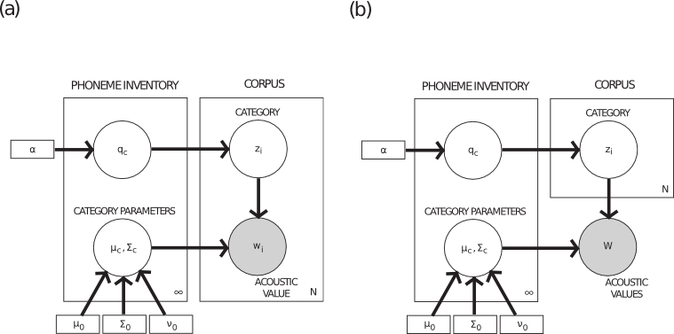
Figure 2: (a) A graphical model of the infinite mixture model. (b) Adapting the model to take into account coarticulation between neighboring sounds.

To estimate the likelihood of a new category, 10 sets of category parameters are sampled from the \(\alpha\) . The likelihood can prior distribution on \(\mu_c\) and \(\sigma_c\), and these are each assigned pseudocounts of 10 be computed for each of these tables as though it were an existing category. If the \(z_i\) being sampled is the only instance of a particular category currently assigned in the corpus, then the parameters from that category are used in place of one of the 10 samples from the prior [9].

The parameters \(\mu_c\) and \(\sigma_c\) should then be resampled for each category, but I could not figure out how to do this, because of the dependencies between different acoustic values. I suspect there is a way to find the posterior on \(\mu_c\) with fixed \(\sigma_c\), which I could not figure out within the time frame for this project, but I’m not sure there is a straightforward way to find the posterior on \(\sigma_c\) at all. In the simulations below I did not ever resample the parameters for existing categories, and any new parameters had to be selected by creating a new category.

Simulations

Simulations compared the coarticulation model to the infinite mixture model. For both models, the concentration parameter \(alpha\) was set at 0.1, and the prior over phonetic categories had parameters \(\mu_0 = 0, \sigma_0 = 0.1, and \nu_0 = 0.1\). The coarticulation model was given a fixed parameter of \(\sigma_S = 0.05\). The samplers were each run for 2,000 iterations. For each simulation, pairwise accuracy and completeness measures were used to compute an overall F-score.

Simulation 1 was conducted to demonstrate that the model can take coarticulatory influences into account, finding the correct categories like a regular infinite mixture model but with greater accuracy in category parameters. This is a non-trivial accomplishment because the category parameters are never resampled in the coarticulation model, whereas they are resampled in the infinite mixture model.

One hundred datapoints were generated from two categories with means at -1 and 1 and variances of 0.01. Each category had a mixing probability of \(\frac{1}{2}\) . \(\sigma_S\) was set at 0.05. The resulting corpus is shown in Figure 3.

Both models recovered the two categories perfectly, and assigned sounds to their respective categories correctly, achieving an F-score of 1. However, the learned category parameters were more accurate in the coarticulation model, where the parameters were \(\mu = 1.05, \sigma = 0.01 and \mu = −0.98, \sigma = 0.01\). The infinite mixture model did substantially worse, recovering \(\mu = 0.72, \sigma = 0.03 and \mu = −0.69, \sigma = 0.02\).

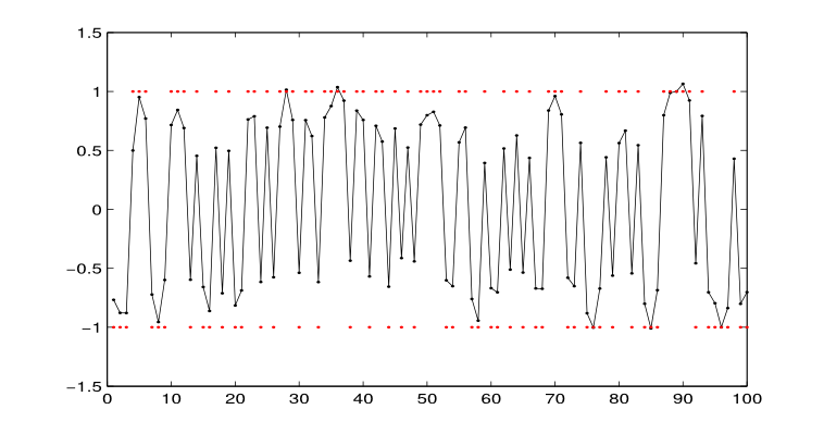
Figure 3: Corpus used for Simulation 1. Connected black dots represent the speech sounds in the corpus, and red dots show the means of the categories that generated the sounds.

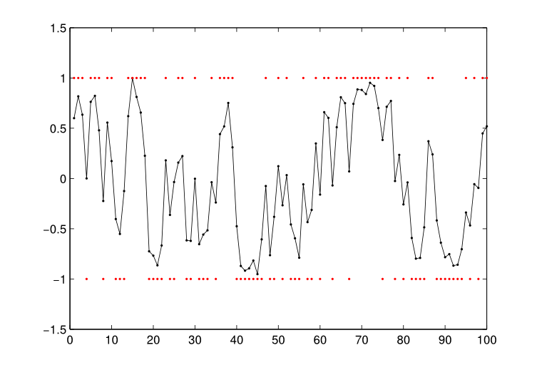
Figure 4: Corpus used for Simulation 2. Connected black dots represent the speech sounds in the corpus, and red dots show the means of the categories that generated the sounds.

Simulation 2 was a more difficult problem, for which the infinite mixture model could not distinguish two categories. This corpus was created using the same parameters as the previous corpus, but the categories in this corpus had variance 0.5, equal to the coarticulatory variance. This corpus is shown in Figure 4.

The infinite mixture model failed to separate the two categories, instead assigning all sounds to a single category with \(\mu_c = −0.03, \sigma_c = 0.34\). This corresponded to an F-score of 0.66. The coarticulation model also found an incorrect number of categories, separating the points into three categories, corresponding to parameters \(\mu_c = −0.91, \sigma_c = 0.06, \mu_c = 0.97, \sigma_c = 0.04, and \mu_c = −0.04, \sigma_c = 0.001\). However, this last category contained only 7 of the 100 sounds in the corpus. This solution had an F-score of 0.93.

Finally, Simulation 3 tested the models on a more complex corpus created from five categories with more substantial overlap. Sounds were generated from categories with means at -2, -1, 0, 1, and 2. Variances were all set to 0.01, like in Simulation 1. However, because the categories were closer together, and because there were more of them, this was a more difficult learning problem. The corpus is shown in Figure 5. The infinite mixture model merged all five categories into a single categories with \(\mu_c = −0.04, \sigma_c = 1.06\), achieving an F-score of 0.33. The coarticulation model found six categories, with the following parameters:

\[\begin{split}\mu_c &= &0.02, &\sigma_c &= 0.01&\\ \mu_c &= &2.06, &\sigma_c &= 0.03&\\ \mu_c &= −&1.85, &\sigma_c &= 0.02&\\ \mu_c &= −&1.08, &\sigma_c &= 0.01&\\ \mu_c &= &0.75, &\sigma_c &= 0.01&\\ \mu_c &= −&2.52, &\sigma_c &= 11.71&\end{split}\]

The last category appears spurious, and indeed contained only 3 sounds from the corpus. This solution had an F-score of 0.89.

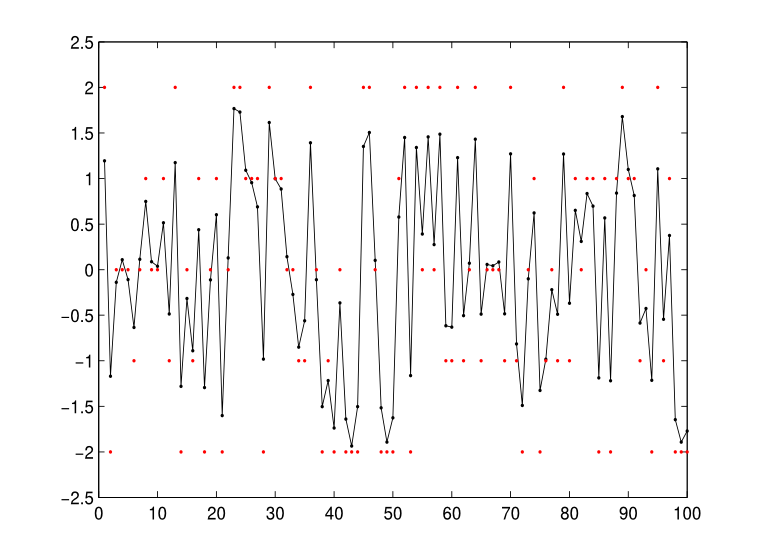
Figure 5: Corpus used for Simulation 3. Connected black dots represent the speech sounds in the corpus, and red dots show the means of the categories that generated the sounds.

Discussion

This project explored the phonetic category learning problem in a system with coarticulation, where sounds are affected by neighboring sounds. Despite a poor inference algorithm in which no category parameters were resampled for existing categories, the coarticulation model showed the ability to recover parameters of phonetic categories in a toy corpus, recovering more accurate parameters than the infinite mixture model and separating categories that were merged by the infinite mixture model.

Immediate future work should address inference of category parameters, finding a way to recover the posterior distribution on µc and \(\sigma_c\) without the need to invert an NxN matrix. It is likely possible to find the posterior distribution on \(\mu_c\) given a fixed value of \(\sigma_c\) , as the degree of contribution of neighboring sounds changes only with changes in sigma_c .

Language learners need to solve several problems at once: learning category assignments and parameters, but also learning the particular coarticulatory patterns of their language, and sequential dependencies between categories. Dependencies between neighboring categories have been especially difficult to deal with because most work in phonetic category acquisition has used exchangeable models, which by definition assign equal probability to any ordering of sounds in the corpus. This paper has proposed a framework for sequential dependences in which these dependencies are characterized by interacting weighted constraints, following work in formal linguistics [6, 8], and has begun exploring the type of inference that can be performed in such a model.

References

[1]	Gautam K. Vallabha, James L. McClelland, Ferran Pons, Janet F. Werker, and Shigeaki Amano. Unsupervised learning of vowel categories from infant-directed speech. Proceedings of the National Academy of Sciences, 104:13273–13278, 2007.

[2]	Bob McMurray, Richard N. Aslin, and Joseph C. Toscano. Statistical learning of phonetic categories: insights from a computational approach. Developmental Science, 12(3):369–378, 2009.

[3]

(1, 2, 3) Naomi H. Feldman, Thomas L. Griffiths, and James L. Morgan. Learning phonetic categories by learning a lexicon. In N. A. Taatgen and H. van Rijnst, editors, Proceedings of the 31st Annual Conference of the Cognitive Science Society, pages 2208–2213. Cognitive Science Society, Austin, TX, 2009.

[4]	James L. Hillenbrand, Michael J. Clark, and Terrance M. Nearey. Effects of consonant environment on vowel formant patterns. Journal of the Acoustical Society of America, 109(2):748–763, 2001.

[5]	(1, 2) Brian Dillon, Ewan Dunbar, and William Idsardi. A single-stage approach to learning phonological categories: Insights from inuktitut. in preparation.

[6]	(1, 2) Legendre, Y. Miyata, and P. Smolensky. Harmonic grammar: A formal multi-level connectionist theory of linguistic well-formedness: Theoretical foundations. Technical Report 90-5, Institute of Cognitive Science, University of Colorado, 1990.

[7]	Sharon Goldwater and Mark Johnson. Learning OT constraint rankings using a maximum entropy model. Proceedings of the Workshop on Variation within Optimality Theory, 2003.

[8]	(1, 2, 3) Edward Flemming. Scalar and categorical phenomena in a unified model of phonetics and phonology. Phonology, 18:7–44, 2001.

[9]	Radford M. Neal. Markov chain sampling methods for Dirichlet process mixture models. Technical Report No. 9815, Department of Statistics, University of Toronto, 1998.